Predictive Analytics - (LAB PROGRAMS)

---

Aim:

☛   ARIMA - Stock market data

Solution :

---

Library Installation:

To install required library files, Open Command Prompt or Terminal and execute the following commands

$ pip install scikit-learn

$ pip install pandas

$ pip install matplotlib

$ pip install statsmodels

---

Dataset (stock_data.csv) :

Date,Open,High,Low,Close,Adj Close,Volume
2015-01-02,26.778,27.240,26.564,27.004,23.404,24742002
2015-01-05,27.073,27.487,26.901,27.060,23.452,26967002
2015-01-06,27.118,27.264,26.684,27.029,23.424,23850002
2015-01-07,27.183,27.450,26.959,27.254,23.607,25516002
2015-01-08,27.387,27.717,27.093,27.486,23.815,2877100
2015-01-09,27.500,27.850,27.300,27.700,24.000,3000000
2015-01-12,27.800,28.100,27.600,27.950,24.200,3100000
2015-01-13,28.000,28.300,27.900,28.150,24.350,3200000
2015-01-14,28.200,28.500,28.000,28.400,24.600,3300000
2015-01-15,28.500,28.900,28.300,28.700,24.900,3400000
2015-01-16,28.800,29.000,28.500,28.900,25.100,3500000
2015-01-19,29.000,29.200,28.700,29.100,25.300,3600000
2015-01-20,29.100,29.500,28.900,29.400,25.600,3700000
2015-01-21,29.300,29.700,29.100,29.600,25.800,3800000
2015-01-22,29.500,29.900,29.300,29.900,26.000,3900000

---

PROGRAM: (ARIMA.py)

 
import pandas as pd
import matplotlib.pyplot as plt
from sklearn.metrics import mean_squared_error
from statsmodels.tsa.arima.model import ARIMA

# Load stock data
df = pd.read_csv("stock_data.csv")

# Convert Date column to datetime and set it as index
df['Date'] = pd.to_datetime(df['Date'])
df.set_index('Date', inplace=True)

# Select Close price
close = df['Close']

# Split data into training and testing sets (80% train, 20% test)
train_size = int(len(close) * 0.8)
train = close[:train_size]
test = close[train_size:]

# Build ARIMA model
model = ARIMA(train, order=(5,1,0))
model_fit = model.fit()

# Forecast for the test period
predictions = model_fit.forecast(steps=len(test))

# Plot Actual vs Predicted Closing Prices
plt.figure(figsize=(10,5))
plt.plot(test.index, test, label='Actual Close Price', marker='o')
plt.plot(test.index, predictions, label='Predicted Close Price', marker='x')
plt.title("ARIMA Stock Price Prediction")
plt.xlabel("Date")
plt.ylabel("Close Price")
plt.legend()
plt.grid(True)
plt.show()

# Calculate Mean Squared Error
mse = mean_squared_error(test, predictions)
print("Mean Squared Error:", mse)

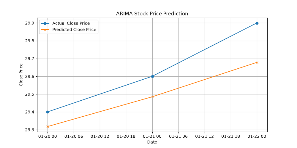
OUTPUT:

 
Mean Squared Error: 0.023058181372076592

---

---

Related Content :

1. Simple Linear regression.   View Solution

2. Multiple Linear regression.   View Solution

3. Logistic Regression.   View Solution

4. CHAID.   View Solution

5. CART.   View Solution

6. ARIMA - stock market data.   View Solution

7. Exponential Smoothing.   View Solution

8. Hierarchical clustering.   View Solution

9. Ward's method of clustering.   View Solution

10. Crowdsource predictive analytics- Netflix data.   View Solution

---