Creating Graphs
To begin, we will look at the foundational function for creating graphs:
plot().
The plot() function
The plot() function is the basic and most commonly used function in R for creating graphs.
Syntax:plot(x, y, type, main, xlab, ylab, col, pch)In the above syntax,
- x, y : Coordinates
- type : Graph type ("p" for points, "l" for line, "b" for both, "n" for nothing)
- main : Title of the graph
- xlab : Label for X-axis
- ylab : Label for Y-axis
- col : Color of the graph
- pch : Shape of the points
Creating a Basic Plot
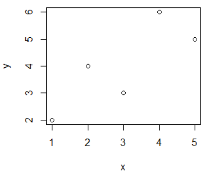
Creating a basic plot using only x and y coordinates.
Example:> x <- c(1, 2, 3, 4, 5)
> y <- c(2, 4, 3, 6, 5)
> plot(x, y)
Adding a Title
Adding a title for the graph using the main argument.
Example:> x <- c(1, 2, 3, 4, 5)
> y <- c(2, 4, 3, 6, 5)
> plot(x, y, main="Basic Plot")

Adding Labels for X and Y axis
Adding labels for the X and Y axis using the xlab and ylab arguments.
Example:> x <- c(1, 2, 3, 4, 5)
> y <- c(2, 4, 3, 6, 5)
> plot(x, y, main="Basic Plot", xlab="Overs", ylab="Runs")

Graph Type
You can create different types of graphs using the type argument. The type argument has different possible values. Those are "p" for points, "l" for line, "b" for both, "n" for nothing. By default, the graph type is points (p).
Example: type = "l"> x <- c(1, 2, 3, 4, 5)
> y <- c(2, 4, 3, 6, 5)
> plot(x, y, main="Basic Plot", xlab="Overs", ylab="Runs", type="l")

> x <- c(1, 2, 3, 4, 5)
> y <- c(2, 4, 3, 6, 5)
> plot(x, y, main="Basic Plot", xlab="Overs", ylab="Runs", type="b")

Color of the graph
You can specify the color of the graph using the col argument. By default, the color is "black".
Example:> x <- c(1, 2, 3, 4, 5)
> y <- c(2, 4, 3, 6, 5)
> plot(x, y, main="Basic Plot", xlab="Overs", ylab="Runs", type="b", col="red")

Shape of the points
You can specify the shape of the points using the pch argument. By default, the shape of the points is "circle". The possible values for pch are from 1 to 25.
Example:> x <- c(1, 2, 3, 4, 5)
> y <- c(2, 4, 3, 6, 5)
> plot(x, y, main="Basic Plot", xlab="Overs", ylab="Runs", type="b", col="red", pch="3")

Adding Lines: The abline() Function
The abline() function is short for "add line". It is used to add horizontal, vertical, or regression lines to an existing plot.
Syntax:abline(a, b, col, lty, lwd)In the above syntax,
- a : Intercept of the line (for y = a + b*x)
- b : Slope of the line
- col : Color of the line
- lty : Line type (solid, dashed, etc.)
- lwd : Line width (thickness)
Add a Regression Line to a Scatter Plot
Example:> x <- 1:10
> y <- 2 * x + 1 + rnorm(10) # y = 2x + 1 with some noise
> plot(x, y, main = "Regression Line", pch = 16)
> abline(lm(y ~ x), col = "red", lwd = 2)

In the above code, lm(y ~ x) fits a linear model; abline() draws that line.
Add a Horizontal Line
> abline(h = 10, col = "blue", lty = 2)
In this, h = 10 adds a horizontal line at y = 10 with a blue dashed line.

Add a Vertical Line
> abline(v = 4, col = "green", lty = 3)
In this, v = 4 adds a vertical line at x = 4 with a green dotted line.

Starting a New Graph While Keeping the Old Ones
Each time you call plot(), directly or indirectly, the current graph window
will be replaced by the new one. If you don't want that to happen, use the command for
your operating system:
- On Linux systems, call X11().
- On a Mac, call macintosh().
- On Windows, call windows().
For instance, suppose you wish to plot two histograms of vectors x and y and view them side by side. On a Windows system, you would type the following:
> x <- c(5,2,1,2,4)
> y <- c(4,5,4,2,1)
> hist(x)
> windows()
> hist(y)

Two Density Estimates on the Same Graph
Plotting two density estimates on the same graph is a very common and useful technique in R, especially to compare the distributions of two datasets. For this, we use the density() and lines() functions.
Example:> exam1 <- c(78,88,92,56,46,64)
> exam2 <- c(63,52,36,82,94,45)
> d1 = density(exam1, from=0, to=100)
> d2 = density(exam2, from=0, to=100)
> plot(d1, main="Density", xlab="Scores", col="red")In the above code, first we compute nonparametric density estimates from the two variables (exam1 and exam2), saving them in objects d1 and d2 by using the density() function. We then call plot() to draw the curve for exam1, at which point the plot looks like below.

We then call lines() to add exam2's curve to the graph, at which point the plot looks like below.
> lines(d2, col="blue")
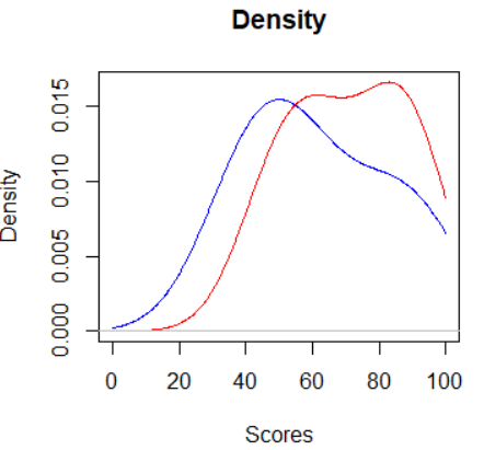
The plot() function starts the graph and also draws the first curve. Then, the lines() function is used to add the second curve on top of the same graph.
Adding a Legend: The legend() Function
The legend() function is used to add a legend to a multicurve graph. This could tell the viewer something like, "The red curve is for exam1, and the blue curve displays the data for exam2."
Syntax:legend(pos, legend, col, lty, lwd, ...)In the above syntax,
- pos : Position of the legend (like "topright")
- legend : A vector of labels
- col : Colors of lines or points
- lty : Line type (1 = solid, 2 = dashed, etc.)
- lwd : Line width
> exam1 <- c(78,88,92,56,46,64)
> exam2 <- c(63,52,36,82,94,45)
> d1 = density(exam1, from = 0, to = 100)
> d2 = density(exam2, from = 0, to = 100)

# Plot first density
> plot(d1, main = "Density", xlab = "Scores", col = "red", lwd = 2)

# Add second density
> lines(d2, col = "blue", lwd = 2)

# Add legend
> legend("topleft", legend = c("Exam 1", "Exam 2"), col = c("red", "blue"), lty = 1, lwd = 2)

Adding Text: The text() Function
The text() function is used to add labels or custom text to specific locations on a plot.
Syntax:text(x, y, labels, col, pos, cex, ...)In the above syntax,
- x, y : Location on the plot where the text goes
- labels : The text you want to show
- col : Text color
- pos : Position relative to the point (1 = below, 2 = left, 3 = above, 4 = right)
- cex : Text size (default is 1)
> exam1 <- c(78,88,92,56,46,64)
> exam2 <- c(63,52,36,82,94,45)
> d1 = density(exam1, from = 0, to = 100)
> d2 = density(exam2, from = 0, to = 100)

> # Plot first density
> plot(d1, main = "Density", xlab = "Scores", col = "red", lwd = 2)

> # Add second density
> lines(d2, col = "blue", lwd = 2)

> # Adding text to lines
> text(20, 0.010, "Exam 1", col = "blue")
> text(42, 0.005, "Exam 2", col = "red")
